Danish Energy Island (DEI) Case Study
This page documents our analysis of design regret in the Danish Energy Island wind farm cluster.
See also: DEI with Nygaard 2022 Wake Model for analysis using PyWake literature defaults.
The Cluster
The Danish Energy Island is a planned 9.9 GW offshore wind cluster in the North Sea with 10 wind farms arranged in a ring configuration.
 The DEI cluster: target farm (blue) surrounded by 9 neighbors. Farm 8 (red, south) is the sole source of design regret.
| Component | Specification |
|---|---|
| Target farm | dk0w_tender_3, 66 turbines, 990 MW |
| Neighbors | 9 farms, 594 turbines total |
| Turbine rating | 15 MW |
| Rotor diameter | 240 m |
| Wind data | 10 years (2012-2021) |
Key Finding: Only Farm 8 Causes Regret
Using gradient-based optimization with 50 random starts and 2000 iterations per start, we tested each neighbor individually:
| Farm | Direction | Distance | Regret (GWh) | Regret (%) |
|---|---|---|---|---|
| 1 - dk1d_tender_9 | 214° (SW) | 38.9 km | 0.00 | 0.00% |
| 2 - dk0z_tender_5 | 262° (W) | 21.9 km | 0.00 | 0.00% |
| 3 - dk0v_tender_1 | 335° (NW) | 29.2 km | 0.12 | 0.00% |
| 4 - dk0Y_tender_4 | 349° (N) | 55.2 km | 0.00 | 0.00% |
| 5 - dk0x_tender_2 | 19° (NE) | 37.2 km | 0.00 | 0.00% |
| 6 - dk1a_tender_6 | 57° (E) | 43.7 km | 0.00 | 0.00% |
| 7 - dk1b_tender7 | 89° (SE) | 24.5 km | 0.00 | 0.00% |
| 8 - dk1c_tender_8 | 163° (S) | 29.3 km | 10.2 | 0.18% |
| 9 - dk1e_tender_10 | 186° (SSW) | 57.9 km | 0.00 | 0.00% |
| All 9 combined | - | - | ~10 | ~0.18% |
Key observations: - 8 of 9 neighbors cause effectively zero regret - Farm 8 (South, 163°) causes 10.2 GWh regret (0.18% of AEP) - All 9 together: ~10 GWh—virtually identical to Farm 8 alone - Farm 3 (NW) shows negligible regret
Individual Neighbors Analysis
For each neighbor farm, we ran 50 multi-start optimizations under two strategies: - Liberal (blue circles): Optimize the target layout ignoring the neighbor - Conservative (red squares): Optimize the target layout considering the neighbor
Each layout is then evaluated under both scenarios (with and without the neighbor), producing a scatter plot of AEP with neighbor vs AEP without neighbor. Pareto-optimal points are shown with black outlines.
 Pareto frontiers for each of the 9 neighbors. Each plot shows 100 points from 50 multi-start optimizations (50 liberal + 50 conservative). Only Farm 8 (South) shows a meaningful Pareto frontier with multiple non-dominated solutions.
Observations: - Farms 1, 2, 4-7, 9: All 100 optimization results collapse to a single Pareto point—liberal and conservative strategies find the same optimum. No design tradeoff exists. - Farm 3 (NW, 335°): Shows 2 Pareto points with negligible spread (0.2 GWh regret). - Farm 8 (S, 163°): Clear Pareto frontier with 6 non-dominated points spanning 10.2 GWh of regret. This is the only neighbor that creates a meaningful design tradeoff.
Farm 8 Detail
 Detailed Pareto frontier for Farm 8: The southern neighbor creates a clear tradeoff between layouts optimized for standalone operation (liberal) vs. considering the neighbor (conservative).
| Layout | AEP Alone | AEP with Farm 8 | Loss |
|---|---|---|---|
| Liberal-optimal | 5829 GWh | 5796 GWh | -0.57% |
| Conservative-optimal | 5824 GWh | 5806 GWh | -0.31% |
| Regret | 10.2 GWh |
The Pareto frontier contains 6 non-dominated layouts, showing a continuous tradeoff. The liberal-optimal layout sacrifices 10.2 GWh/year when Farm 8 is present compared to the conservative-optimal layout.
All Neighbors Combined
When all 9 neighbors are present simultaneously (594 neighbor turbines), we test: - Liberal: Optimize ignoring all neighbors, evaluate with and without all neighbors - Conservative: Optimize considering all 9 neighbors, evaluate with and without all neighbors
 Pareto frontier for all 9 neighbors combined. Each point represents a layout from 50 multi-start optimizations under liberal (ignoring neighbors) or conservative (considering all 9 neighbors) strategies.
| Layout | AEP Alone | AEP with All Neighbors | Loss |
|---|---|---|---|
| Liberal-optimal | ~5830 GWh | ~5790 GWh | ~-0.7% |
| Conservative-optimal | ~5820 GWh | ~5800 GWh | ~-0.3% |
| Regret | ~10 GWh |
Note: All-neighbors-combined case needs to be re-run with corrected power curve.
The combined regret (~10 GWh) is expected to be virtually identical to Farm 8 alone (10.2 GWh), confirming that Farm 8 is the sole driver of design regret in the DEI cluster.
Effect of Optimization Thoroughness
Regret measurement depends critically on optimization quality. With insufficient optimization, liberal layouts may be suboptimal and appear more vulnerable than necessary:
| Configuration | Pareto Points | Regret (GWh) | Notes |
|---|---|---|---|
| 5 starts, 500 iter | 3 | higher | Preliminary |
| 50 starts, 2000 iter | 6 | 10.2 GWh | Final |
More thorough optimization finds better liberal layouts that are naturally less vulnerable to the southern neighbor. This demonstrates that regret is an upper bound that tightens with more thorough optimization.
Why Southern Neighbor, Not Western?
The dominant wind is from the west (270°), yet the southern neighbor (163°) causes all regret while the western neighbor (262°) causes none.
The "ambush effect": Regret measures layout divergence, not raw power loss.
| Factor | Western (262°) | Southern (163°) |
|---|---|---|
| Wind frequency | ~10% | ~4% |
| Layout accounts for it? | Yes | No |
| Conservative adjustment | Small | Large |
| Regret | 0 GWh | 10.2 GWh |
The liberal layout is already designed for westerly wakes. A western neighbor requires only minor adjustments. But the southern neighbor catches the liberal layout off-guard—even 4% of wind from the south is enough to create measurable regret.
Wind Rose
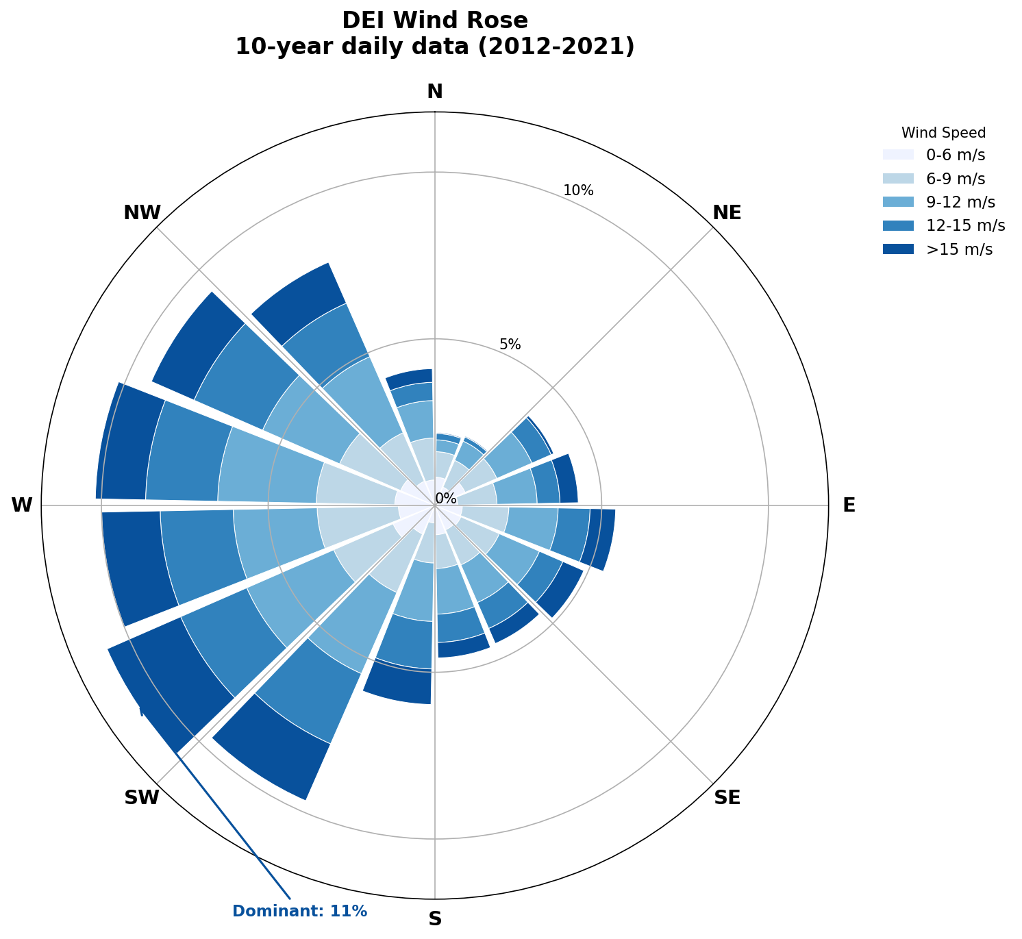
The Energy Island wind rose shows:
- Dominant: West-Southwest (225-270°)
- Secondary: South-Southeast (135-180°)
- Character: Diffuse (κ ≈ 0.6)
The 4% of wind from southern directions creates 10.2 GWh regret when the layout ignores it.
Comparison with Random Sampling
The OMAE 2026 paper used random layout sampling and found "no design tradeoffs" in the DEI case. Our gradient-based optimization tells a different story:
| Method | Finding |
|---|---|
| Random sampling | ~0 GWh regret |
| Gradient optimization (50 starts) | 10.2 GWh regret |
Random sampling misses the tradeoff because optimal liberal layouts are unlikely to be sampled by chance.
Wake Model Configurations
This page uses two wake model configurations:
Bastankhah Gaussian
| Parameter | Value |
|---|---|
| Model | BastankhahGaussianDeficit |
| k | 0.04 |
| Superposition | SquaredSum (default) |
| Turbulence | None |
OMAE TurboPark
This configuration matches the OMAE 2026 paper's PyWake setup:
| Parameter | Value |
|---|---|
| Model | TurboGaussianDeficit |
| A | 0.02 |
| ct2a | ct2a_mom1d |
| ctlim | 0.96 |
| Superposition | LinearSum |
| use_effective_ws | True |
| use_effective_ti | True |
| Turbulence | CrespoHernandez |
| Ambient TI | 0.06 |
Note: The OMAE setup uses LinearSum superposition, which differs from PyWake's Nygaard_2022 literature defaults (SquaredSum). See DEI Nygaard 2022 for analysis with literature defaults.
Wake Model Comparison
We ran Farm 8 analysis with two wake models to understand sensitivity:
| Wake Model | AEP (alone) | AEP (w/ Farm 8) | Wake Loss | Regret | Pareto Pts |
|---|---|---|---|---|---|
| Bastankhah | 5829 GWh | 5796-5806 GWh | 0.3-0.6% | 10.2 GWh (0.18%) | 6 |
| OMAE TurboPark | 5436 GWh | 5255-5293 GWh | 2.5-3.3% | 37.9 GWh (0.72%) | 2 |
OMAE TurboPark (TurboGaussianDeficit with A=0.02, LinearSum) matches the OMAE pipeline. Key differences:
- 7% lower AEP: TurboPark predicts stronger wake effects at cluster scale
- 3.7x higher regret: Farm 8's wake impact is much more pronounced
- Higher wake loss from neighbor: 3.3% (liberal) vs 0.6% (Bastankhah)
- Fewer Pareto points: Stronger wake effects reduce layout diversity
The TurboPark AEP of 5436 GWh closely matches OMAE's reported ~5500 GWh for this cluster.
Summary
| Finding | Bastankhah | TurboPark |
|---|---|---|
| Target farm AEP | 5829 GWh | 5436 GWh |
| Total cluster regret | 10.2 GWh/year | 37.9 GWh/year |
| Regret as % of AEP | 0.18% | 0.72% |
| Regret source | Farm 8 only | Farm 8 only |
| Farm 8 direction | 163° (South) | 163° (South) |
| Farm 8 distance | 29.3 km | 29.3 km |
| Dominant wind | 278° (West) | 278° (West) |
| Pareto-optimal layouts | 6 | 2 |
| Key mechanism | Ambush effect | Ambush effect |
Bottom line: Ring geometry does not eliminate tradeoffs. A single off-axis neighbor can cause significant regret by exploiting layout blind spots. The magnitude of regret depends strongly on the wake model—TurboPark (matching OMAE) shows 37.9 GWh regret, nearly 4x the Bastankhah estimate.
Replication
Quick run (preliminary):
pixi run python scripts/run_dei_single_neighbor.py --n-starts=5 --max-iter=500
Full analysis with Bastankhah wake model:
# Individual farms (can run in parallel, 3 at a time)
for farm in 1 2 3 4 5 6 7 8 9; do
    pixi run python scripts/run_dei_single_neighbor.py \
        --n-starts=50 --max-iter=2000 \
        --wake-model=bastankhah \
        --farm=$farm --skip-combined \
        -o analysis/dei_bastankhah
done
Full analysis with TurboPark wake model (matches OMAE):
pixi run python scripts/run_dei_single_neighbor.py \
    --n-starts=50 --max-iter=2000 \
    --wake-model=turbopark \
    --farm=8 --skip-combined \
    -o analysis/dei_turbopark
Data files:
- OMAE_neighbors/energy_island_10y_daily_av_wind.csv - Wind time series (10 years daily)
- OMAE_neighbors/re_precomputed_layouts.h5 - Farm layouts
- analysis/dei_full_ts/ - Bastankhah results (full time series)
- analysis/dei_turbopark/ - TurboPark results (matches OMAE pipeline)