Methodology
Problem Setup
Target Wind Farm
- Size: 16 turbines in a 16D × 16D square area
- Rotor diameter (D): 200 m
- Hub height: 120 m
- Rated power: 10 MW per turbine
- Minimum spacing: 4D (800 m)
Neighboring Farm Representation
Potential neighboring farms are represented as "blobs" - morphable shapes defined by B-spline boundaries with 4 control points. For each analysis run, we randomly sample multiple blob configurations to explore how different neighbor geometries affect design tradeoffs.
Important: The blob shapes are randomly sampled, not optimized to find worst-case configurations. This Monte Carlo approach provides a distribution of possible regret values across different neighbor geometries, but does not guarantee finding the absolute worst-case scenario.
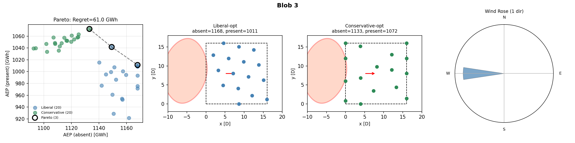 Example blob (coral/red region) positioned upwind of the target farm (dashed rectangle). Turbines within the blob create wakes that affect the target farm.
Blob Sampling Parameters
- Position: Center sampled within (-10D to -4D, 0.2L to 0.8L) where L = target size
- Size: Radius sampled between 5D and 10D
- Shape: Aspect ratio sampled between 0.6 and 1.6
- Number of blobs: 20 random configurations per wind rose type
Wake Model
We use the Bastankhah Gaussian deficit model with:
- Turbulence intensity factor: k = 0.04
- Superposition: Root-sum-of-squares (SquaredSum) by default; LinearSum available via
--superposition linearsum
The Annual Energy Production (AEP) is computed as:
where \(P_i\) is the power curve, \(U_{i,d}\) is the effective wind speed at turbine \(i\) for direction \(d\), and \(w_d\) is the probability weight.
Wind Rose Types
Von Mises Distribution
The Von Mises distribution is the circular analog of the normal distribution:
where: - \(\mu\) = mean direction (270° = West) - \(\kappa\) = concentration parameter - \(I_0\) = modified Bessel function of order 0
| κ value | Interpretation |
|---|---|
| 0 | Uniform distribution |
| 1 | Mild concentration |
| 2 | Moderate (typical offshore) |
| 4+ | High concentration |
Wind Rose Configurations Tested
| Type | Description | Parameters |
|---|---|---|
| Single | Unidirectional | 270° only |
| Uniform | Omnidirectional | 24 directions, equal weights |
| Von Mises κ=1 | Diffuse | μ=270°, 24 directions |
| Von Mises κ=2 | Moderate | μ=270°, 24 directions |
| Von Mises κ=4 | Concentrated | μ=270°, 24 directions |
| Bimodal | Two peaks | 270° (70%) + 90° (30%) |
Optimization Methodology
What Is Optimized vs. Sampled
| Component | Method | Description |
|---|---|---|
| Blob shape | Random sampling | B-spline control points sampled from bounded distributions |
| Neighbor positions | Fixed grid | 25 potential positions on a 5×5 grid, masked by blob |
| Target layout | SGD optimization | Turbine positions optimized via gradient descent |
Pooled Multi-Start Approach
For each randomly sampled blob configuration, we run a pooled multi-start optimization on the target farm layout only:
- Liberal Strategy (20 starts): Optimize target layout assuming neighbors are absent
- Objective: Maximize AEP_absent
-
Gradient-based optimization with random initialization
-
Conservative Strategy (20 starts): Optimize target layout accounting for neighbor wakes
- Objective: Maximize AEP_present
-
Same optimization procedure
-
Cross-Evaluation: All 40 layouts are evaluated under both scenarios
-
Pareto Analysis: Identify non-dominated layouts
SGD Optimization Settings
SGDSettings(
    max_iter=3000,      # For single direction
    # max_iter=2000,    # For 24 directions
    learning_rate=D/5,  # 40 m step size
)
Constraint Handling
- Boundary constraints: Soft penalty for turbines outside target area
- Spacing constraints: Soft penalty for turbines closer than 4D
- Gradient projection: Ensures feasibility during optimization
Regret Computation
Pareto Frontier
A layout is Pareto-optimal if no other layout achieves both: - Higher AEP when neighbors are absent, AND - Higher AEP when neighbors are present
Regret Definition
- Liberal-optimal: Layout optimized to maximize AEP without neighbors (i.e., designed in isolation), then evaluated with neighbors present
- Conservative-optimal: Layout optimized to maximize AEP with neighbors present
Both terms are evaluated under the same conditions (neighbors present). The regret isolates the design effect: how much AEP is lost by having designed in ignorance of the neighbors, not the total AEP impact of the neighbors themselves.
If regret > 0, there exists a fundamental tradeoff between the two objectives.
Convergence Verification
To ensure results are not artifacts of insufficient optimization, we verified convergence by varying the number of random starts:
| Configuration | n=5 | n=10 | n=20 | n=40 |
|---|---|---|---|---|
| Single direction | 53.70 | 38.62 | 41.15 | 38.62 |
| Uniform | 24.27 | 24.27 | 20.29 | 20.29 |
| Von Mises κ=4 | 16.69 | 17.75 | 9.77 | 9.77 |
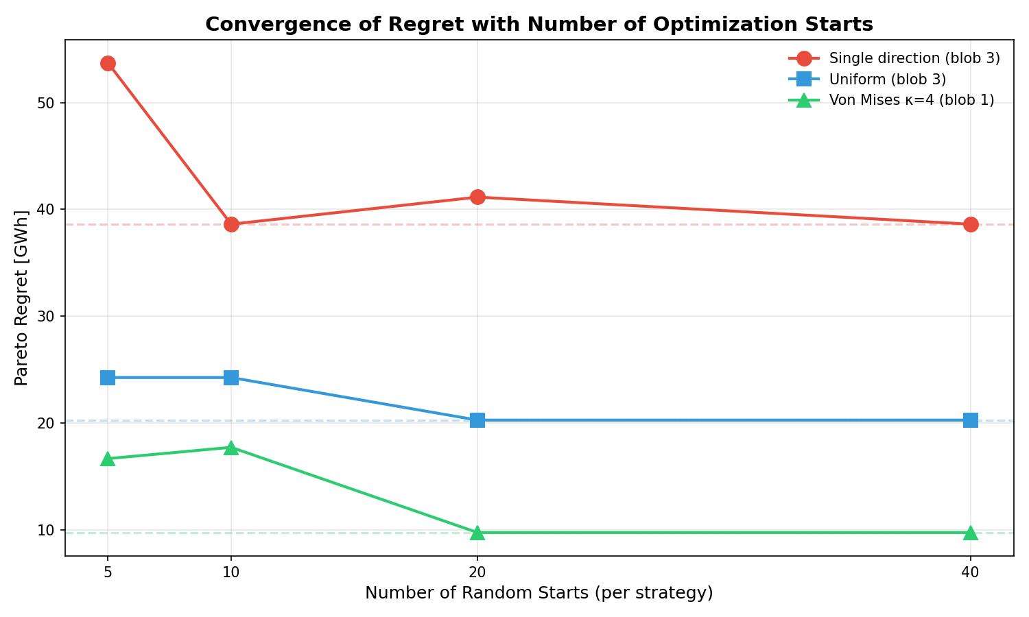
Results stabilize by n=20 starts per strategy. The full analysis uses n=20.